REGIONAL
PROTECTION IN
FINAL
REPORT
Evgenia
Kolomak
Institute
of Economics and Industrial Engineering Siberian Branch of Russian Academy
of Sciences, 17, pr. Academica Lavrentieva,
E-mail:
kolomak@online.sinor.ru
Introduction
Regional leaders are inclined to interference
in the regulation of local economy everywhere in
Tools of the regional protection include
tax exemptions, credits, subsidies, budget compensations. As federal budget
subsidies decreased in
Very often the regional authorities explain the price control, subsidizing and granting tax exemptions to local producers by social imperatives. However several facts contradict to this thesis. A characteristic of the regional budgets is high level of overdue for salary and transfers to population (more 40%), the next item is overdue to infrastructure monopolies, supplying public utilities (28%) (Report of the World Bank (2000)). Hence, the biggest part of burden, resulted form regional policy is imposed on population.
In this paper we study why the regional
authorities in
Why policy-makers intervene in a market? Review of literature
Government intervention into market
is discussed in different topics. For our problem three of them are of special
interest: political constrains of transition period, interest groups, and
attitudes towards governments.
Although price liberalization is a
key element of transition and is a necessary condition of the market mechanism
and for improvement in the allocation of resources (Lipton and Sachs (1990),
Boyko (1992), McKinnon (1991)) the political constrains of the transition
period may make a gradual price reform preferable despite its efficiency
costs (Dewatripont and Roland (1992 a, b), Roland (2000)). What policy-makers
put in place depends on the political acceptability of the reforms. Milder
reforms and even reversal sometimes are the only way to speed up the process
and enhance political acceptability.
Political constrains affecting the
speed and design of price reforms are determined by initial conditions. Kruegel
and Ciolko (1996) and Castanheira and Popov (1999) suggest that the rate
and extend of price liberalization may be endogenous. The worse the initial
conditions for transformation the greater the probability of the deep transformation
recession as a result of the liberalization, and hence there are more likely
delays in liberalization. When initial conditions are favorable, rapid liberalization
is feasible and preferable.
The political constrains are reinforced when the fact that bureaucrats and regulators may benefit from the persistence of price control is taken into account. Shliefer and Vishny (1992) show that price control creates rent for state sector and represents opportunities for soliciting bribes from interest groups.
The role of lobby groups in the shape of trade policy is incorporated into analysis in two ways. The first approach stresses political competition between opposing candidates. In the works of Magee et al. (1989), Hillman and Ursprung (1988), the lobby groups evaluate their prospects under the alternative trade policy proposals have been made by competing parties. In making their giving decisions, the lobbies weigh the benefit of an increasing the probability of their favorite party being elected against the direct cost for the donation. The parties use the resources to influence the election outcome. In the second approach presented in Stigler (1971), Hillman (1982), Grossman and Helpman (1994), the economic policy is considered as being set by an incumbent government seeking to maximize its political support. The political support function has as arguments the welfare that designated interest groups derive from the chosen policies and the deadweight loss that the policies impose on society at large. In this formulation, campaign contributions do not enter directly into the analysis, and the political competition of the next election is kept in the background. Both of the approaches consider the political optimization as underlying the endogenous determination of trade policy.
Features of the regional policy in Russia
Local policy depends also on the attitudes towards the governments. Paper by Edwards and Keen (1996) synthesizes the two extremes: the view of government as a Leviathan and the view of government as a benevolent maximiser of their citizens’ welfare. The policy-makers have preferences defined over some item of public expenditures which, while financed from general revenues, benefits only the policy-maker, and the welfare of their representative citizen. Polishchuk (2000) shows that under certain assumptions a revenue-maximizing Leviathan-type government might offer better conditions for economic development than a benevolent, which is concerned about economic well-being of its constituency at large.
So a design of regional protection policy is a result of a number of factors, among which are initial conditions, political process, influence of interest groups, and objectives of the policy-makers. Based on the results of the reviewed studies we propose a model of regional trade policy determination.
A
Model
Statement of the
problem
We consider a regional market, so
we may assume that the economy is small and market regulation is the result
of the political process. One of the attitudes of Russian regional economies
is a high level of specialization in the production, the producers have incentives
to form lobby groups and they demonstrate ability to overcome the free-rider
problem.
The regional lobby groups confront
regional policy-makers with requirements to provide protection for the sector
against external producers in exchange for political support. The regional
government bears costs for implementing an inefficient protection policy
that is result of creating deadweight loss and its accountability to the
general electorate. The government sets protection policy comparing benefits
of the political cooperation with local producers and costs of deterioration
of its reelection prospects. The implemented policy must be financially feasible.
The proposed theoretical framework for the analysis of the barriers of regional price regulation is very similar to the one developed by Grossman and Helpman (1994) in the study devoted to protection trade policy.
Overview of Grossman
- Helpman’s results
Grossman and Helpman consider a small,
competitive economy. Free trade is efficient for such an economy, so any
policy interventions can be ascribed to the political process. They assume
that there is a high degree of concentration in the ownership of the specific
inputs and that the various owners of some these inputs have banded together
to form lobby groups. They assume also that some factor owners overcome the
free-rider problem to conduct joint lobbying activity, while other do not.
The lobby groups may offer political
contributions to the incumbent politicians, who are in a position to set
the current trade policy. While the lobby groups ignore the effects of their
contributions on the election probabilities, the incumbent politicians may
see a relationship between total collections and their reelection prospects.
Incumbent politicians’ objective is to maximize a weighted sum of total political
contributions and aggregate social welfare.
The authors model the lobbing process
as follows. Each interest group confronts the government with a contribution
schedule. The schedule maps every policy vector that the government might
choose (where policies are import and export taxes and subsidies) into a
campaign contribution level. The government then sets a policy vector and
collects the contribution associated with its choice.
Let introduce some notations: p is the vector of domestic prices; Ci(p) - the contribution schedule
tendered by lobby i; Wi(p) - gross-of-contributions joint welfare of the members
of lobby group i; G(p) -
government’s utility function; L – set of sectors which are
able to organize a lobby group.
The authors are interested in the
political equilibrium of a two-stage non-cooperative game in which the lobbies
simultaneously choose their political contribution schedules in the first
stage and the government sets policy in the second. An equilibrium is a set
of contribution functions {Ci0(p)}, one for each organized lobby group, such that each
one maximizes the joint welfare of the group’s members given the schedules
set by the other groups and the anticipated political optimization by the
government; and a domestic price vector p0 that
maximizes the government’s objective taking the contribution schedules as
given. The Nash-equilibrium contribution schedules implement an equilibrium
policy choice.
Grossman - Helpman’s model has the
structure of a menu-auction problem. Bernheim and Whinston (1986) have characterized
the equilibrium for a class of such problems. Grossman and Helpman applied
these results to the problem of protection trade policy. The adaptation resulted
in following proposition.
Proposition 1. ({Ci0}iÎL, p0}) is a subgame-perfect Nash equilibrium
of the trade policy game if and only if:
(i) Ci0
is feasible for all iÎL;
(ii) p0 maximizes G(p) on the set of domestic price vector;
(iii) p0 maximizes Wj(p) - Cj0(p)+ G(p) on the set of domestic price vector for every jÎL;
(iv) for every jÎL there exists a pj that maximizes G(p) on the set of domestic price vector such that Cj0(pj)=0.
Condition (i) states that lobby’s contributions must be nonnegative and no greater than the joint income available to the sector. Condition (ii) states that, given the political contributions offered by the lobbies, the government sets trade policy to maximize its own welfare. Condition (iii) stipulates that for every lobby, the equilibrium price vector must maximize the joint welfare of that lobby and the government, given the contributions offered by other lobbies. Condition (iv) requires that for every lobby j there must exist a policy that elicits a contribution of zero from lobby j, which the government finds equally attractive as the equilibrium policy p0. If there does not exist such a policy, then lobby j can lower their political contributions without changing the government’s choice, what of necessity leave sector j strictly better off.
Condition (iii) characterizes the equilibrium structure of protection. Condition (iv) characterizes the equilibrium structure of political contributions.
Our problem and one of Grossman - Helpman are very similar and we largely rely on the significant results obtained by the authors, however there are several differences. The differences come from three issues. The first one is the fact that Russian regional governments can not use export and import tariffs and subsidies opposed to the case of Grossman - Helpman consideration and are restricted to other tools of price regulation: price ceiling, price mark-ups, input and output subsidies, tax exemptions or credits. The second issue stems from the requirement of financial acceptability of the regional protection policy, regional budget constrain needs explicit introduction into the model. The third difference is explained by the statement of problem to distinguish between different tools of the protection policy. These differences modify Grossman - Helpman‘s model and obviously its analytical inferences as well.
Formal framework
We consider a regional market with
tradable goods i=0,1,…,n. The local demand curve for a particular
good is di(pi). Assume when there is
no price dispersion all consumers prefer domestic goods. Suppose
that in the absence of trade the equilibrium price of goods i=1,…,n
is higher than in the situation of interregional and/or international trade.
Assume that there is no possibility for the protection of good 0. Let use
good 0 as a numeraire, and let its price equal to 1, p0=1.
The supply curves of local producers depend on input and output exogenous prices and/or implemented local protection policy. Assume the regional government can use input, output subsidies and tax exemptions. We assume that production in each sector requires labor and a specific input, subsidized are and regulated are prices of the specific inputs. Consequently the supply function of a locally produced good i depends on price (which differs form the exogenous market price if local government imposes price limitations), input subsidy, output subsidy, input price restrictions, and tax exemption yi(pi, si,ri,ti) where pi is exogenous price, si is subsidy per unit of good i, ri is subsidy per unit of specific input in sector i, and ti - tax exemptions granted to sector i. Let denote by p, s, r,, t the vectors of output prices, output and input subsidies, and tax exemptions respectively.
Let the regional economy is populated by individuals with identical preferences. Each individual maximizes utility given by
![]() (1)
(1)
where x0
is consumption of good 0 and xi is consumption
of good i, i=1,…,n. With these quasi-linear preferences demand
for good i is independent of the prices of other goods, and
possibilities for substitutions of complementarities among the goods are
absent. An individual spending an amount E consumes xi=di(pi) of good i, i=1,…,n, where the demand function is inverse of ui¢(xi), and ![]() .
.
The consumer surplus derived from the goods is equal to
![]() (2)
(2)
Where p is the vector
of the exogenous prices.
The protection must
be financially acceptable. The financial acceptability means satisfying the
budget constrain, local government expenditures should be less than receipts.
The receipts are in the form of taxation of the domestic aggregate income,
the expenditure items are input and output subsidies to local producers.
The excess of receipt over protection expenditures, here regarded as a source
of public expenditures financing, is:
 (3)
(3)
Where t
is the tax rate, zi(pi, si,
ri, ti) - demand for specific
input in sector i, and b reflects the local
government ability to ‘soften’ local budget, it can be done through transferring
expenses of local policy to another budgets or by obtaining additional resources
from higher level budgets.
The producers are interested in protection
for their sectors and enter the political activity. The lobby representing
a sector i makes its political contribution contingent on
the protection policy implemented by the government. Denote by ci(pi,si,ri,ti) the contribution tendered by lobby
i. The lobby determines the contributions to maximize total
welfare of the sector’s members: labor income plus profit of the sector plus
consumer surplus and benefits from the public expenditures less contributions.
The scheme of the distribution of the political donations among the sector’s
members is out of consideration here. We assume the existence of ways to
allow all the members to share the gains from the political coordination.
The joint gross-of-contribution welfare of the members of sector i is:
 (4)
(4)
Where pl - the wage rate; pi* - exogenous price of the specific input in sector
i; ai - share of the voting population
related to sector i.
The government’s utility function
depends on attitudes towards government. There are two extreme types of government
presented in the literature as stark alternatives: benevolent and Leviathan.
When the government is a benevolent, it is a maximizer of their citizens’
welfare. A Leviathan – government maximizes items of expenditures benefit
only the policy-makers. A more general assumption is that policy-makers are
neither wholly benevolent nor wholly self-serving, an obvious encompassing
is that the policy-makers maximize a weighted sum of citizens’ welfare and
their own wellbeing. The latter assumption is accepted for our problem.
The incumbent government maximizes
a weighted sum of political contributions and aggregate welfare of the population.
The political contributions provide direct benefits to the government. However
the social welfare can result in indirect benefits if voters are more likely
to reelect a government that provides a high standard of living. The government
objective function is:
![]() (5)
(5)
Where 0£q£1.
We consider a two-stage non-cooperative
game: in the first stage sector’s lobbies make decision and propose political
contributions contingent on protection policy; in the second stage the regional
government determine the implemented policy. An equilibrium is a set of contribution
functions {ci0(pi,si,ri,ti)}, one for each sector, such that
each one maximizes the joint welfare of the sector’s members given the schedules
proposed by the other sectors and the anticipated optimization by the regional
government; and a regional protection policy vector (pi0,si0,ri0,ti0)
that maximizes
the government’s objective taking the contribution schedules as given. The
Nash-equilibrium realizes an equilibrium policy.
The proposed formal framework corresponds
to the structure of Grossman-Helpman’s problem. However the modification
of the Grossman-Helpman’s model and more detailed consideration of some issues
modify Proposition 1. The proposition relevant to our problem is as follows.
Proposition 2. ({ci0}iÎL, {p0,s0,r0,t0}) is a subgame-perfect Nash equilibrium
of the regional protection policy game if and only if:
(a) {ci0}
is feasible for all iÎL;
(b) {p0,s0,r0,t0} maximizes G(p,s,r,t) subject to budget constrain r(s,r)³0 for all iÎL;
(c) {p0,s0,r0,t0} maximizes Wj(p,s,r,t)+ G(p,s,r,t) subject to budget constrain r(s,r)³0 for every jÎL;
(d) for every jÎL there exists a bundle (pj,sj,rj,tj) that maximizes G(p,s,r,t) subject to budget constrain
such that cj0(pj,sj,rj,tj)=0.
Condition (a) implies that lobby’s proposals are positive and less than welfare of members of the represented sector. Condition (b) states that given the political proposals of the interest groups the government determines input and output subsidies, tax exemptions maximizing its utility function and satisfying the budget constrain taking into account exogenous price of output. Condition (c) stipulates that for every sector the equilibrium bundle of input and output subsidies, tax exemptions, and price of output maximizes sum of welfare of the sector and the government, given the budget constrain and the proposals of other lobbies. Condition (d) means that for every sector j participating in the political lobbing there exists a combination of subsidies, tax exemptions, and output price, which requires contribution of zero from sector j, and which is equivalent for the government to equilibrium protection policy.
The equilibrium structure of protection policy
Grossman and Helpman have proved that if the contribution schedules are differentiable around the equilibrium, the shape of the political contributions reveal the lobbies’ true preferences in the neighborhood of the equilibrium. They have also demonstrated an interesting property of Nash equilibria, in equilibrium government behaves as if it attributed to lobbies higher weigh than other population. Below we show that these results hold to our model as well.
Let assume that the political contribution
functions and welfare functions are differentiable. To characterize the structure
of the equilibrium protection policy let consider conditions (b) and (c)
Proposition 2, they imply that the first order condition is satisfied at
{p0,s0,r0,t0}:
![]() (6)
(6)
![]() (7)
(7)
Where l is a Lagrange multiplier. Inserting (7) into (6) gives ![]() .
By definition (4)
.
By definition (4) ![]() .
Taken together the equations imply
.
Taken together the equations imply
![]() (8)
(8)
Equation (8) establishes that around the equilibrium change in the political contributions reflects the effect of change of the government protection policy on the joint welfare of members of the lobby’s group.
By the definition (4) ![]() ,
where Wi(p0,s0,r0,t0) is net-of-contribution welfare of group i members.
If the political contributions correspond to true preferences of the group,
than Wi(p0,s0,r0,t0)³Wi((p,s,r,t) and
,
where Wi(p0,s0,r0,t0) is net-of-contribution welfare of group i members.
If the political contributions correspond to true preferences of the group,
than Wi(p0,s0,r0,t0)³Wi((p,s,r,t) and
![]() (9)
(9)
Condition (b) of Proposition 2 states that if (p0,s0,r0,t0) and (p,s,r,t) are feasible than
![]() ,
or
,
or
![]() .
.
From expression (9)
![]() .
.
Consequently the government in the equilibrium maximizes weighted sum of welfare of different groups of population. Welfare of groups of population presented by lobbies in the political process receives weight (1+q), welfare of other ones receives weigh q, where 0£q£1.
Further let present in a more
detailed record expression (7), it takes form
![]() .
.
Inserting (8) into the expression gives
![]() (10)
(10)
The equation shows how marginal change of protection policy influences the welfare of the groups of populations distinguishing between participating in lobbing and do not participating.
So the properties of the equilibrium structure of the regional protection policy are as follows. Firstly, around equilibrium the political contributions reveal preferences of the interest groups regarding protection policy. Secondly, equilibrium protection policy results in distribution of welfare in favor of the sectors, participating into political lobbing. Thirdly, in equilibrium marginal change of welfare of different groups influenced by the protection policy depends on the fact of participating in political lobbing.
We consider further properties of the different protection tools: output subsidies, input subsidies, or tax exemptions. Let first consider output subsidies
a) Output subsidies
We analyze a solution of equation
(10).
From (4) we find
![]() ,
,
where sij - Kronecker’s symbol. Substitution of the terms in expressions
(10) allows to derive
![]()
![]()
Let introduce an indicator variable ji that equals 1 if the sector uses lobby pressure and 0 - otherwise.
Denote
![]()
by
L*. The equation takes the form
![]() .
.
From (3) we find
![]() .
.
Inserting let to derive
 ,
,
where ejs - subsidy elasticity
of production good j. Let
![]() ,
,
then

Proposition 3. The government in the equilibrium chooses output subsidies that satisfy
for all j=1,…,n
So output subsidies for a good positively correlated with tax rate, ability of the regional administration to soften regional budget constrain, with weight attributed to population’s welfare, exogenous input price, with lobbing activity of the sector and overall lobbing pressure of the regional producers. Output subsidy for a particular good negatively correlated with level of exogenous output price, subsidy elasticity of production, granted tax exemptions and input subsidies.
In contrast with Grossman – Helpman’s economy, where export and import tariffs are considered, our case is restricted to positive subsidies. International trade policy belongs to federal level jurisdiction and regional authorities have not to interfere with this sphere.
Output subsidies are positive
if
![]() .
.
Assume
![]()
and k>0, the latter requires λ-L-θ>0,
what means that the regional authority have tight budget, at least enough
tight to take the budget into consideration when the government faces pressure
from population and lobbing groups. When the budget is not binding restriction
of the policy-making, the government may grant any subsidies and any tax
exemptions, it is not the case of our analysis.
The first term in of the above expression is always positive, the second one is always negative, and sign of the third one depends on technology and input and output prices. So granting output subsidies to a producer depends on input subsidies, tax exemptions to the producer, on ration of input and output exogenous prices and technology of the production.
The range of output subsidies values is presented in Diagram 1
Diagram 1
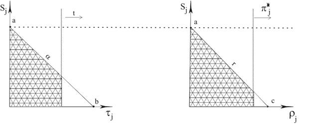
Here slope
![]() ,
,
slope
 ,
,
![]() ,
,
![]()
(b may be less or more than t),

(c may be less or more than π*j).
b) Input subsidies
We continue analysis of the equation (10).
From equation (4)
![]() ,
,
equation (10) takes form:

Or
![]() .
.
From (3) we can find
![]() .
.
Taken together let us derive
 ,
,
where ejr - input price subsidy elasticity of demand for input of production
good j.
Proposition 4. The government in the equilibrium chooses input subsidies that satisfy
for all j=1,…,n
So input subsidies for a good positively correlate with level of the exogenous input price, with tax rate, weight attributed to population’s welfare, ability of the regional administration to soften regional budget constrains and lobbing activity. However level of input subsidy for a particular good negatively correlate with output exogenous price, with input price subsidy elasticity of demand for input, with tax exemptions and output subsidies to the sector.
If we assume that k>0,
then input subsidies are positive if
![]() .
.
The first and the second terms in the expression are positive, the third
term is negative.
So probability of input subsidy granting depends on ratio of tax exemption to tax level in the region, on level of exogenous input price and output price, on granted output subsidies, on technology and tightness of the regional budget constrain.
The range of input subsidies values is shown in Diagram 2
Diagram 2
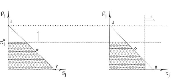
Here slope
![]() ,
,
slope
 ,
,

(d may be less or more than π*j),  ,
,
 (g may be less or more than t).
c) Tax exemptions
This case concludes the analysis of equation (10).
From (4) we find
![]() .
.
Substitution of the terms in expressions (10) let us to derive
![]()
![]()
The equation takes the form
![]() .
.
From (3) we find
![]() .
.
Inserting lets to derive
 ,
,
where ejt - tax exemption elasticity
of production good j.
Proposition 5. The government in the equilibrium chooses tax exemptions that satisfy
for all j=1,…,n
So tax exemptions for a sector positively correlate with tax rate, with weight attributed to population’s welfare, with lobbing activity of the sector and with input exogenous price. Tax exemptions for a sector negatively correlate with level of exogenous output price, tax exemption elasticity of the production, input and output subsidies granted to the sector.
Diagram 3
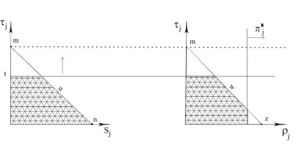
Here slope
![]() ,
,
slope
 ,
,

(m may be less or more than t),
![]() ,
,
![]()
(z may be less or more than π*j).
The table below summarizes the characteristics of the equilibrium protection policy.
Table 1. The correlation
characteristics of equilibrium
|
Variables |
Output subsidy |
Input subsidy |
Tax exemption |
|
Output subsidy |
|
- |
- |
|
Input subsidy |
- |
|
- |
|
Tax exemption |
- |
- |
|
|
Tax rate |
+ |
+ |
+ |
|
Exogenous output price |
- |
- |
- |
|
Exogenous input price |
+ |
+ |
+ |
|
Weight attributed to population’s welfare |
+ |
+ |
+ |
|
Overall lobbing pressure on a regional government |
+ |
+ |
+ |
|
Political activity of the sector’s lobby |
+ |
+ |
+ |
|
Output subsidy elasticity of production |
- |
|
|
|
Input price subsidy elasticity of demand for input |
|
- |
|
|
Tax exemption elasticity of production |
|
|
- |
|
Ability of the regional administration to soften regional budget constrain |
+ |
+ |
+ |
Empirical estimations
A. Hypotheses
Assuming the model is correct the empirical estimations will support the hypotheses as follows.
Hypothesis 1.
Output subsidies, input subsidies and tax exemptions are substituting tools
of the regional protection. Each of the measures negatively correlates with
others.
To
test this hypothesis correlation of subsidies and tax exemptions will be
estimated.
Hypothesis 2. Regional
subsidizing and granting tax exemptions is a feature of the regions having
higher tax burden in the regions.
For
testing these hypotheses connection between subsidies, tax exemptions and
level of the regional tax collection must be estimated.
Hypothesis 3. Regions
demonstrating active subsidizing and granting tax exemptions have larger
share of transfers from the federal center what is one of the way to soften
.regional budget constrain.
To
test the hypothesis the dependence of subsidies and tax exemptions on level
of federal transfers received by region has to be estimated.
Hypothesis 4. Subsidizing
and granting tax exemptions positively correlated with political lobbing
of the interest groups.
Lobbying
power depends on the concentration of the producer’s interests; the higher
is the concentration the higher is the ability to influence the government
and to persuade it of the protection. To test the hypothesis the correlation
of the regional subsidizing and tax exemptions with level of the regional
specialization should be estimated. Usually the agreements between policy-makers
and business have a long-term character, so an autoregressive dependence
worth to take into account.
Hypothesis 5. Activity
of the regional protection depends on needs of the population, in the model
the corresponding indicator is weight attributed to the population’s welfare.
Some literature considers industry protection as result of social policy,
the protection is granted to industries that would, otherwise, be declining.
One of the possible consequences of decline is unemployment; correlations
of the protection activity with level of unemployment will be estimated.
Hypothesis 6. Subsidies
and tax exemptions depend on exogenous prices, so macroeconomic demand and
supply shocks result in sharp change of the prices may also result in change
of protection activity. There were two years in the recent period in Russia
are famous for sharp devaluation of ruble, growth of consumer demand and
prices of goods of both import and domestic production: 1995 and 1998. Correlations
of the protection activity with macroeconomic price indexes and two macro-shock
dummy variables for 1995 and 1998 will be estimated.
Hypothesis 7. Statistical
data on subsidies and tax exemptions allows to assume extension of the regional
protection practice in the considered years. So time trend needs to be included.
B. Information
Testing
of the formulated hypotheses assumes data for a period of time on subsidies,
tax exemptions, and import by regions and by sectors, and information on
structure of economies, on budgets, and taxes by regions.
Reports
on the executed regional budgets for 1996 - 2000 are taken from Ministry
of Finance of the
However
the disaggregated information on subsidies by 10 sectors[1]
was obtained only for
Table
2 Appendix 2 presents summary statistics for subsidies and tax exemptions
data set on Russian regions. Tax exemptions variable for Russian regions
is constructed assuming that three types of tax relief might be a result
of lobbing activity: tax relief for particular enterprises, tax relief for
industries and setting up free economic zones. Any of these tax reliefs contributes
1 to the tax exemptions variable, so the variable takes values from 0 to
3, the former corresponds to case of no tax relief, the latter means granting
three types of the mentioned ones.
In
order to test the formulated hypotheses under the conditions of the restricted
information we estimated two systems. Each of the systems is a modification
of one corresponding to the system of the advanced above hypotheses.
C. Methods of estimation
Initial system
The theoretical model structure implies
to do an empirical analysis by sectors and by regions. Because of radical
changes during transition period in
 (A)
(A)
 (B)
(B)
Where:
m r, u r, hr - fixed regional effect;
nrt, x rt, yrt - random regional error;
eirt - random sector’s error;
Subsidiesirt - subsidies for sector i from regional budget in region r in year
t;
Dummies for yearst - dummy year variables;
Level of taxationrt - tax income per capita in total
regional budget income in region r in year t;
Transfersrt - share of transfers from federal
budget in the regional budget income in region r in year
t;
Share in regional productionirt - share of sector i in
production of region r in year t;
Exogenous priceit - average price level for sector’s
i production in year t;
Tax exemptionsirt - tax exemptions for sectors i provided by regional government in region r
in year t;
Unemploymentrt - share of unemployed active population
in region r in year t;
Time trendt – number of year t.
As
it is mentioned above quantitative data for subsidies and tax exemptions
by sectors were obtained for one region -
The
modified system adapted for one region is as follows:
Modification 1
 (A’)
(A’)
 (B’)
(B’)
Subscript
i identifies sector, t – year; λi and
φi are
sector’s effects.
However
effect of the omitted regional variables (unemployment, federal transfers,
and regional level of taxation) is of interest as well, in order to estimate
their contribution the estimations were done on the basis of aggregated by
sector data. The information on tax exemption is another as well; it is fact
of tax granting. Variable of tax exemptions is equal to number of decisions
on tax exemptions adopted in a region. Variable of share of industry in regional
production have to be omitted, since sum of the shares for a region is equal
one. However as a proxy for lobbing pressure in a region dummy variable of
specialization level is introduced, which takes value “1” when there is an
industry producing more than 1/3 of total regional industrial product and
value “0” other wise. Variable of exogenous price in the aggregated by sectors
case coincides with time effect. The observations have the panel structure
and include characteristics of 88 regions over time period 1996 – 2000. Since
1995 is not in the covered period, one dummy variable for macro-shock in 1998
is used in the estimations.
Modification 2
 (A’’)
(A’’)
 (B’’)
(B’’)
Comments
on the new notations are below.
Subsidiesrt - share of subsidies for the local
producers in regional budget expenditures in region r in
year t;
Specialization levelrt - dummy variable for the specialization
level, which takes value “1” when there is an industry producing more than
1/3 of total regional industrial product in region r in year
t and value “0” other wise;
Tax exemptionsrt - number of decisions granted different
tax exemptions in region r in year t;
λr and μr - regional effects.
The
equations (A’), (B’), (A’’), and (B’’) are dynamic panel regressions with
endogenous variables. One of the proposed methods for such models is the
two-step Arellano and Bond (1991) GMM estimator, where past variables are
used as instruments.
For
instance consider equation (A’), where i=1,…,10, t=1,…,8.
For convenience, we introduce the following notations: yit –
subsidiesit,
vector xit –
vector of independent variables in it equation (A’). So we
have yit=δ yi,t-1+ xit’β+λi+υit. Instruments
for yit are
yis,
where s<t, instruments for xit are
xis,
where s<t. Define


The
matrix of instruments is W=[W1`,…, W10`]. The
preliminary first-step consistent estimator:

Differenced
residuals obtained from the preliminary estimator:
![]() .
.
Define
![]()
The
resulting estimator is:

A
consistent estimate of the asymptotic variance of the coefficients is given
by

The
same way of estimation is used for equations (B’) and (A’’) – (B’’).
D. Results of the
estimations
The
correlation characteristics for systems (A’)-(B’) and (A’’)-(B’’) are presented
in tables 3 - 4 Appendix 2 correspondingly.
The
results of the empirical estimations are presented in the tables below.
Table
2. The results of regression (A’) estimation
|
Variables |
Coefficient |
P-value |
|
Constant |
-4.86 |
0.228 |
|
Dummy for macroeconomic
shock 1995 |
3.91 |
0.038 |
|
Dummy for macroeconomic
shock 1998 |
1.39 |
0.060 |
|
Time linear trend |
1.61 |
0.001 |
|
Share in regional
production |
0.07 |
0.439 |
|
Exogenous price |
-0.01 |
0.975 |
|
Tax exemptions |
-0.11 |
0.518 |
|
Subsidies in the
previous year |
0.08 |
0.034 |
|
R2 |
0.32 |
|
So
the significant and positive is correlation of the subsidies provided for
the sectors with subsidies of the previous year and macroeconomic price shocks.
There was increasing tendency in subsidizing local producers, time variable
is positive and significant. Other variables were insignificant for
Table
3. The results of regression (B’) estimation
|
Variables |
Coefficient |
P-value |
|
Constant |
1.65 |
0.560 |
|
Dummy for macroeconomic
shock 1995 |
2.85 |
0.031 |
|
Dummy for macroeconomic
shock 1998 |
0.50 |
0.078 |
|
Time linear trend |
0.65 |
0.006 |
|
Share in regional
production |
0.01 |
0.842 |
|
Exogenous price |
-0.03 |
0.015 |
|
Subsidies |
-0.06 |
0.482 |
|
Tax exemptions
in the previous year |
0.25 |
0.029 |
|
R2 |
0.34 |
|
The
results confirm negative correlation of tax exemptions with exogenous output
price level for the sectors and positive correlation with macroeconomic instability.
There is practice of long-term supporting of the producers in the region,
tax exemptions in the previous year is significant and positive variable.
Wight of the sectors in regional production and provided subsidies are insignificant.
In
the both regressions share of the sectors in the regional production is insignificant
variable so the weight is not matter, the more important is lobbing activity
itself. Subsidies and tax exemptions are granted to the sectors which had
obtained them in the past and continue to keep their positions. One of the
factors of value of subsidies and of tax exemptions is the macroeconomic
situation. Size of subsidies and tax exemptions does not depend on each other.
Table
4. The results of regression (A’’) estimation
|
Variables |
Coefficient |
P-value |
|
Constant |
3.77 |
0.885 |
|
Dummy for macroeconomic
shock 1998 |
0.17 |
0.561 |
|
Time linear trend |
0.11 |
0.016 |
|
Level of taxation |
0.07 |
0.031 |
|
Transfers |
0.45 |
0.093 |
|
Unemployment |
-9.22 |
0.736 |
|
Specialization
level |
0.91 |
0.494 |
|
Tax exemptions |
-0.85 |
0.537 |
|
Subsidies in the
previous year |
0.54 |
0.010 |
|
R2 |
0.29 |
|
Table
5. The results of regression (B’’) estimation
|
Variables |
Coefficient |
P-value |
|
Constant |
0.22 |
0.676 |
|
Dummy for macroeconomic
shock 1998 |
0.09 |
0.597 |
|
Time linear trend |
0.09 |
0.041 |
|
Level of taxation |
0.01 |
0.029 |
|
Transfers |
0.01 |
0.032 |
|
Unemployment |
-0.73 |
0.815 |
|
Specialization
level |
0.23 |
0.437 |
|
Subsidies |
-0.02 |
0.691 |
|
Tax exemptions
in the previous year |
0.60 |
0.000 |
|
R2 |
0.34 |
|
The
estimations on the sample of the aggregated data for
Unemployment
is not significant factor of the regional protection, so the social factor
does not influence the regional governments’ decisions on the protection
of local producers very much. The estimations on the country level sample
have confirmed the results received for one region that the regional authorities
prefer to support the same sectors, significant are correlations with previous
year level of the support. Another common feature is tendency to increase
the protection for local producers through subsidizing and tax relief; both
of the activities have a significant growing trend.
Conclusions
Protection of local producers becomes
one of the typical features of the sub-federal policy in
References
In English
Arellano, M. and S. Bond (1991),
Some Tests of Specification for Panel Data:
Baltagi, B.H. (2001), Econometric
Analysis of Panel Data, 2-nd edition, John Wiley & Sons, LTD.
Bernheim, D. and M. Whinston (1986),
Menu Auctions, Resource Allocation, and Economic Influence, Quarterly Journal
of Economics, vol. 101, N 1, pp. - 31.
Boycko, M. (1992), When Higher Incomes Reduce Welfare:
Queues, Labor Supply, and Macroeconomic Equilibrium in Socialist Economies.
Quarterly Journal of Economics, 107, pp. 907 – 920.
Castanheira, M and V.Popov, (1999), Framework Paper
on the Political Economic of Growth in
Dewatripont, M. and G. Roland (1992a),
Economic Reform and dynamic political constraints, Review of Economic Studies,
59, pp. 703-730.
Dewatripont, M. and G. Roland (1992b), The virtues
of gradualism and legitimacy in the transition to a market economy, Economic
Journal 102, pp. 291 – 300.
Edwards, J., M. Keen, (1996) Tax competition and
Leviathan, European Economic Review, 40, pp. 113 – 134.
Grossman, G. and E. Helpman (1994) Protection for
Sale, American Economic Review, vol. 84, N 4, pp. 833 – 850.
Hilman, A. (1982), Declining Industries
and Political-Support Protectionist Motives, American Economic Review, vol.
72, N 5, pp. 1180-1187.
Hilman, A. and H. Ursprung (1988),
Domestic Politics, Foreign Interests, and International Trade Policy, American
Economic Review, vol. 78, N 4, pp. 729-745.
Hsiao, C. (1986), Analysis of Panel
Data.
Kruegel, G., and M. Ciolko, (1998), A Note on Initial
Conditions and Liberalization during Transition, Journal of Comparative Economics,
26 (4), pp. 618-634.
Lipton, D. and J. Sachs (1990) Creating a Market
Economy in
Magee, S., W. Brock and Y. Leslie, Black hole tariffs
and endogenous policy theory: Political economy in general equilibrium.
McKinnon, R. (1991)
The Order of Economic Liberalization. Financial Control in the Transition
to a Market Economy, The
Polishchuk L. (2000)“Political Economy of Scale
and Endogenous Rule of Law”, mimo,
Roland G. (2000), Transition and Economics: Politics,
Market, and Firms. The MIT Press.
Shliefer, A. and R. Vishny, (1992),
Pervasive shortages under socialism, Rand Journal of Economics 23 N 2, pp.
237 –246.
Stigler ,G. (1971), The Theory of
Economic Regulation,
In
Russian
Gluschenko K.P, (2001), Пространственное поведение уровней цен,
ЭММ, т.37, № 3, с. 3 –13
Report of the World Bank «Destroying of the system
of non-payments in
Henson F. (2001) Effect of the factor of regional diversity on economic transformation in
Appendix
1
Table 1
Subsidies to enterprises
from federal and regional budgets, percent of GNP
|
|
1992 |
1993 |
1994 |
1995 |
1996 |
1997 |
1998 |
|
Subsidies from federal
budget |
5,8 |
2,5 |
3,1 |
2,2 |
1,6 |
1,8 |
1,9 |
|
Subsidies from the
regional budgets |
5,3 |
6,8 |
7,3 |
5,2 |
6,3 |
6,9 |
7,2 |
Source: Russian
Statistical Yearbook, 1999
Table 2
Share of regional
subsidies in the regional budget expenditures, percentage
|
|
Total subsidies |
Subsidies to industry,
agriculture, transport and construction |
|||||||||
|
|
1996 |
1997 |
1998 |
1999 |
2000 |
1996 |
1997 |
1998 |
1999 |
2000 |
|
|
Minimum |
0,0 |
0,0 |
0,0 |
0,0 |
0,0 |
0,0 |
0,0 |
0,0 |
0,0 |
0,0 |
|
|
Maximum |
50,0 |
48,5 |
44,3 |
47,5 |
38,2 |
11,6 |
14,2 |
13,7 |
8,7 |
15,1 |
|
|
Median |
18,9 |
19,0 |
22,8 |
19,1 |
18,8 |
3,9 |
3,6 |
3,9 |
2,8 |
4,8 |
|
|
Average |
18,5 |
18,3 |
21,9 |
18,8 |
19,1 |
4,2 |
4,1 |
4,0 |
3,0 |
5,0 |
|
|
Standard deviation |
10,8 |
9,7 |
9,3 |
7,9 |
8,0 |
3,1 |
3,2 |
2,6 |
2,0 |
2,7 |
|
Source: data of Ministry
of Finance RF
Table 3
Regions granting tax exemptions,
percentage
|
|
1992 |
1993 |
1994 |
1995 |
1996 |
1997 |
1998 |
1999 |
2000 |
2001 |
|
Tax
relief for particular enterprises |
1 |
3 |
8 |
17 |
26 |
26 |
28 |
24 |
19 |
11 |
|
Tax
relief for branches of industry |
1 |
6 |
14 |
25 |
38 |
40 |
47 |
52 |
46 |
43 |
|
Tax
relief for small business |
0 |
1 |
3 |
4 |
11 |
14 |
19 |
20 |
22 |
18 |
|
Free
economic zones |
1 |
1 |
3 |
6 |
7 |
10 |
11 |
7 |
2 |
0 |
|
Tax
relief for investors |
1 |
3 |
4 |
11 |
22 |
51 |
79 |
84 |
89 |
91 |
Source: Legislative data base
«Consultant Plus. Regional Legislation»
Appendix
2
Table 1
Summary statistics
on protection variables for
|
|
Number of observations |
Mean |
Standard deviation
|
Minimum |
Median |
Maximum |
|
Subsidies |
80 |
5.78 |
8.67 |
0 |
1.45 |
32.34 |
|
Tax exemptions |
80 |
3.19 |
6.82 |
0 |
0.15 |
30.93 |
Source: Administration
of
Table 2
Summary statistics
on protection variables for Russian regions
|
|
Number of observations |
Mean |
Standard deviation
|
Minimum |
Median |
Maximum |
|
Subsidies to industry,
agriculture, transport and construction (percentage of regional budget
expenditures)* |
440 |
3.93 |
3.1 |
0 |
3.8 |
15.1 |
|
Tax exemptions** |
440 |
0.46 |
0.65 |
0 |
0 |
3 |
*Source: Ministry
of Finance of RF
** Source: Legislative data base «Consultant Plus.
Regional Legislation»
Table
3
Correlations
of subsidies and tax exemptions in
|
Variables |
Pooled |
Industrial
fixed effects |
Industrial
between effects |
|
Subsidies |
|||
|
Dummy for macroeconomic
shock 1995 |
3.302 [0.000] |
3.302 [0.000] |
- |
|
Dummy for macroeconomic
shock 1998 |
0.259 [0.002] |
0.259 [0.002] |
- |
|
Time linear trend |
1.212 [0.000] |
1.212 [0.000] |
- |
|
Share in regional
production |
0.106 [0.092] |
0.050 [0.104] |
0.277 [0.020] |
|
Exogenous prices |
-0.019 [[0.034] |
-0.019 [0.031] |
-0.027 [0.098] |
|
Tax exemptions |
0.103 [0.299] |
0.125 [0.275] |
0.010 [0.579] |
|
Subsidies in the
previous year |
0.042 [0.043] |
0.014 [0.075] |
0.086 [0.016] |
|
Tax
exemptions |
|||
|
Dummy for macroeconomic
shock 1995 |
1.906 [0.002] |
1.906 [0.002] |
- |
|
Dummy for macroeconomic
shock 1998 |
1.860 [0.003] |
1.860 [0.002] |
- |
|
Time linear trend |
0.828 [0.001] |
0.828 [0.000] |
- |
|
Share in regional
production |
0.010 [0.277] |
0.033 [0.119] |
0.058 [0.149] |
|
Exogenous prices |
-0.025 [0.001] |
-0.024 [0.001] |
-0.175 [0.082] |
|
Subsidies |
0.057 [0.199] |
0.065 [0.153] |
0.008 [0.279] |
|
Tax
exemptions in the previous year |
0.228 [0.023] |
0.196 [0.037] |
0.242 [0.053] |
Table
4
Correlations
of subsidies and tax exemptions in the Russian regions with explanatory variables
|
Variables |
Pooled |
Regional
fixed effects |
Regional
between effects |
|
Subsidies |
|||
|
Dummy for macroeconomic
shock 1998 |
3.188 [0.009] |
3.153 [0.000] |
- |
|
Time linear trend |
0.528 [0.003] |
0.542 [0.000] |
- |
|
Level of taxation |
0.124 [0.019] |
0.111 [0.013] |
0.135 [0.034] |
|
Transfers |
0.144 [0.003] |
0.217 [0.000] |
0.066 [0.041] |
|
Unemployment |
-0.011 [0.092] |
-0.022 [0.331] |
-0.011 [0.131] |
|
Specialization
level |
0.490 [0.346] |
0.573 [0.981] |
0.682 [0.516] |
|
Tax exemptions |
-0.034 [0.933] |
0.659 [0.265] |
-0.420 [0.489] |
|
Subsidies in the
previous year |
0.056 [0.011] |
0.022 [0.046] |
0.078 [0.053] |
|
Tax
exemptions |
|||
|
Dummy for macroeconomic
shock 1998 |
0.495 [0.000] |
0.495 [0.000] |
- |
|
Time linear trend |
0.155 [0.000] |
0.155 [0.000] |
- |
|
Level of taxation |
0.019 [0.035] |
0.001 [0.057] |
0.001 [0.044] |
|
Transfers |
0.014 [0.005] |
0.015 [0.047] |
0.015 [0.049] |
|
Unemployment |
0.002 [0.000] |
0.007 [0.000] |
0.001 [0.218] |
|
Specialization
level |
0.187 [0.573] |
0.259 [0.627] |
0.346 [0.825] |
|
Subsidies |
-0.001 [0.933] |
0.013 [0.265] |
-0.017 [0.489] |
|
Tax exemptions
in the previous year |
0.319 [0.000] |
0.150 [0.002] |
0.907 [0.000] |